2.3 Principal Stresses, Eigenvalues, and Stress Paths

For a particular laboratory test, we could sketch Mohr circles at every point where we measure the stress components. However, doing this is problematic because we typically measure many stress points during an experiment, and plotting so many Mohr circles would be unreasonable. For example, consider an isotropically consolidated triaxial compression test in which the initial effective stress is 50, the cell pressure remains constant at 50, and the vertical stress is increased from 50 to 100. Assume that 50 different stress measurements are made. The Mohr circles associated with such a stress path are plotted in Fig. 2.3.1. This figure contains too much information to be particularly useful. Fortunately, there is a better way to represent such data using “stress paths”. Before we discuss stress paths, we must first discuss principal stresses.

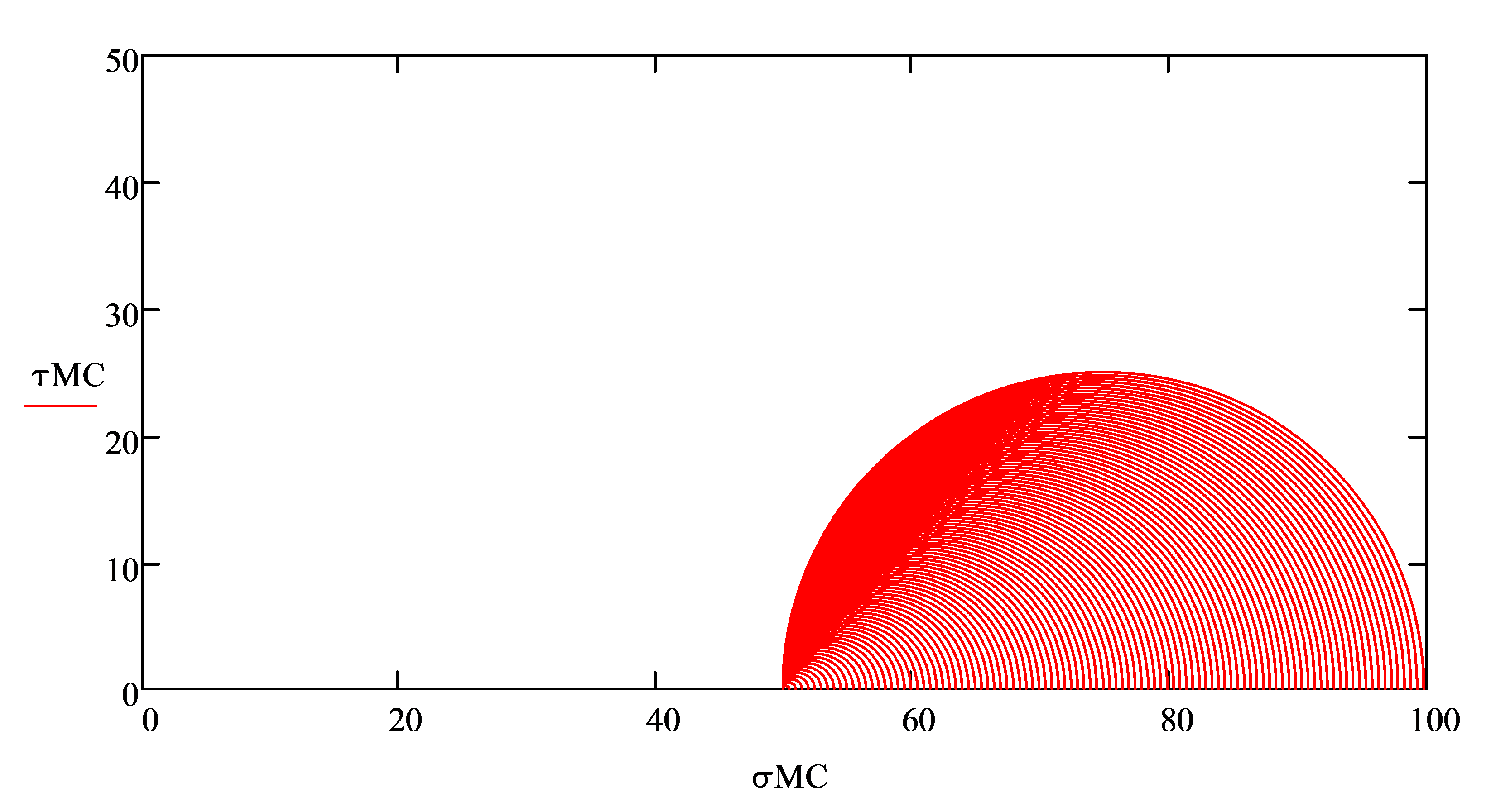
Figure 2.3.1. Mohr circle representation of laboratory test data

2.3.1 Principal Stresses as Eigenvalues

For any Cauchy stress tensor, there exists at least one orientation in which \(\sigma_{ij}\)=0 for i \(\neq\) j, and \(\sigma_{ij} \neq\)0 for i=j (i.e., stresses are non-zero only on the diagonal, and off-diagonal terms are zero). The directions corresponding to this stress state are are called principal stress directions. Consider a principal stress direction corresponding to a unit vector with directions \(n_1, n_2,\) and \(n_3\). The plane normal to this unit vector is called a principal stress plane. Projecting the Cauchy stress tensor onto the principal stress plane results in a normal stress, \(\lambda\), but no shear stresses, acting on the plane as illustrated by the equation below. The normal stress, \(\lambda\) is an Eigenvalue of the Cauchy stress tensor, while the unit vector corresponding to the normal stress, \(n\), is an Eigenvector. Since the Cauchy stress tensor is 3x3, there are three Eigenvalues (the principal stresses) and three corresponding Eigenvectors (the principal stress directions). If the three Eigenvectors are assembled into a 3x3 matrix, the transpose of this matrix is equal to the rotation tensor required to produce a principal stress state. \[\left[ \begin{matrix} \sigma _{11}^{{}} & \sigma _{12}^{{}} & \sigma _{13}^{{}} \\ \sigma _{21}^{{}} & \sigma _{22}^{{}} & \sigma _{23}^{{}} \\ \sigma _{31}^{{}} & \sigma _{32}^{{}} & \sigma _{33}^{{}} \\ \end{matrix} \right]\left[ \begin{matrix} {{n}_{1}} \\ {{n}_{2}} \\ {{n}_{3}} \\ \end{matrix} \right]=\lambda \left[ \begin{matrix} {{n}_{1}} \\ {{n}_{2}} \\ {{n}_{3}} \\ \end{matrix} \right]\]

This is an Eigenvalue problem in which the Eigenvalues correspond to the principal stresses and the Eigenvectors correspond to the principal stress directions. Hence, we can easily compute principal stresses for any Cauchy stress tensor by simply computing the Eigenvalues of the stress tensor. An app for for computing Eigenvalues of a Cauchy stress tensor is available below, and you can also find routines in Matlab, Mathcad, and probably even Excel.

Try it yourself

2.3.2 Stress Invariants, \(p\), \(p^{'}\), and \(q\)

After computing the principal stresses, we may compute stress invariants. These include the mean total stress, \(p,\) the mean effective stress, \(p^{'}\), and the deviator stress, \(q\). The mean total stress is simply the average of the principal stresses:

\[p=\frac{\sigma _{1}+\sigma _{2}+\sigma _{3}}{3}\]

The mean effective stress, \(p'\), is obtained by subtracting the pore pressure \(u\) from the mean total stress or by the Cauchy stress tensor in terms of effective stress rather than total stress:

\[p^{'}=p - u = \frac{\sigma _{1}^{'}+\sigma _{2}^{'}+\sigma _{3}^{'}}{3}\]

The deviator stress is based on differences between the principal stresses, and is therefore an indication of the shear demand placed on the soil:

\[q=\sqrt{\frac{1}{2}\left[ {{\left( {{\sigma }_{1}}-{{\sigma }_{2}} \right)}^{2}}+{{\left( {{\sigma }_{2}}-{{\sigma }_{3}} \right)}^{2}}+{{\left( {{\sigma }_{1}}-{{\sigma }_{3}} \right)}^{2}} \right]}\]

Note that \(q=\sigma_1-\sigma_3\) for triaxial test conditions where \(\sigma_2=\sigma_3\). Also note that \(q\) can be formulated in terms of total stress or effective stress because the pore pressure cancels out.

Plotting \(q\) vs. \(p\) results in a total stress path, while plotting \(q\) vs. \(p^{'}\) results in an effective stress path. Going back to the example of the triaxial test shown in Fig. 2.3.1, we can represent the stress condition using a Cauchy stress tensor defining the initial consolidation condition, \(\sigma_{o}\) and a Cauchy stress tensor defining the change in loading during shearing, \(\Delta\sigma\). The resulting stress path begins at \((p_{o},q_{o}) = (50.0,0.0)\) and ends at \((p_{f},q_{f}) = (66.67,50)\). Try changing the \(\sigma_{o}\) and \(\Delta\sigma\) to plot your own stress paths.